Improving demand planning with a double exponential smoothing model

Accuracy in the demand forecasts for the Sales and Operations Planning (S&OP) process is extremely important and is fundamental to its success within a company. Some shortcomings found in simpler forecasting methodologies may undermine the credibility of your process.

In this article we will explain how to solve some of the issues associated with the simple exponential smoothing model. As seen in a previous blog post, this model creates a simple forecast that assumes that future demand time series is similar to its past. A major issue with this simple smoothing is its inability to identify and project a trend.

Try our fast & simple demand forecasting solution
Sign up for free to SKU Science today!
Pre-loaded sample data - No credit card required

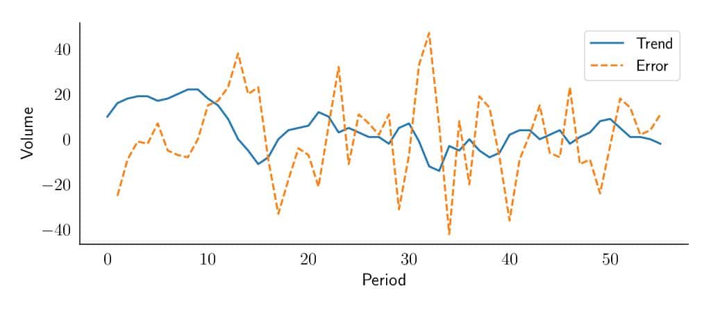
We define the trend as the average variation of the time series level between two consecutive periods. In our November 2018 blog, the level is the average value around which the demand varies over time. So, for example, if you had a sales level last week of 10 pieces, and this week the sales level is around 20 pieces, this means that you have a positive trend of 10 pieces per week.

If you assume that your time series follows a trend, most likely you will not know its magnitude in advance; especially as this magnitude could vary over time. However, there is now a model that can distinguish by itself the trend over time. As seen for the level, this new model will estimate the trend based on a new learning parameter called beta ( $\beta$ ), giving more or less importance to the most recent observations. Remember that alpha ( $\alpha$ ) will determine how much importance is given to the most recent demand observation.

These demand forecasting techniques are now fully available to SKU Science, and we explain some of their key concepts below.

Double exponential smoothing demand forecasting method at a glance

The general idea behind double exponential smoothing models is that both level and trend will be updated at each period based on the most recent observation and the previous estimation of each component.

As you may remember, with the simple exponential smoothing model, we updated the forecast at each period partially based on the previous demand and partially based on the previous forecast.

We will now do the same for both level ( $a_{t}$ ) and trend ( $b_{t}$ ).

Our new demand forecasting model will update its estimation of the level at each period thanks to two pieces of information: the last demand observation and the previous level estimation increased by the trend.

This demand forecasting model will also have to estimate the trend. Just as for the level, it represents how much weight is given to the most recent level observation.

As soon as we are out of the historical demand period, we simply forecast each period as the last forecast plus the trend, and so the model will extrapolate the latest trend it has observed. However, as we will see later, this might present a problem.

You can see below the mathematical representation for the forecasting technique:

Level Estimation: $a_t=\alpha d_{t}+(1-\alpha)( a_{t-1}+b_{t-1})$
Trend Estimation: $b_t=\beta(a_{t}-a_{t-1})+ (1-\beta)b_{t-1}$
Future Forecast: $f_{t+1}=a_{t}+b_{t}$

Initialization of our demand forecasting model

As seen with the forecast initialization of the simple exponential smoothing, we have to discuss how to initialize the first estimations of our level and trend, and we will have two options as depicted below.

Simple initialization

We can initialize the level and the trend simply based on $a_0 = b_0$ and $b_0=d_1 - d_0$ . This is a simple and fair initialization method.

Linear regression

Another way to initialize $a_0$ and $b_0$ would be to do a linear regression of the first n demand observations, that could be defined as an arbitrarily rather low number (e.g. 3 or 5). How to do linear regressions is out of scope for this article.

Insights on these demand forecasting models

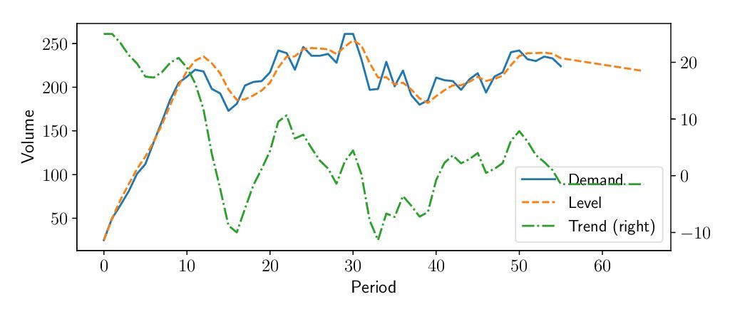
Exponential smoothing models are very useful as they allow us to understand a forecast or a time series thanks to their decomposition between the level and the trend and (as we will see in another blog post), the seasonality. One can check the state of any of the demand sub-components at any point in time, just as you might check what is happening under the hood of a car.

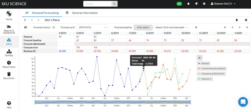
On the example below, we’ve plotted these different components to show you how our model understands a specific product. It explains why our model forecasts a specific value.

The value of the different smoothing parameters will also tell you something about the variability or smoothness of your product. High values will denote a product where each variation should have an impact on the forecast; low values will denote products with a more constant behavior that should not be impacted by short-term fluctuations.

Limitations of the double exponential smoothing demand forecasting model

Our double exponential smoothing model is now able to recognize a trend and extrapolate it into the future. This is a major improvement compared to simple exponential smoothing or moving average. But, unfortunately, this comes with a risk.

Our model will assume that the trend will go on forever. This might result in some issues for mid/long-term forecasts. We will solve this thanks to the damped trend model - a model that was published 25 years ago, in 1985!

Next to the risk of infinite trend, we still have

The lack of seasonality. This will be solved via the triple exponential smoothing model detailed in our next blog post.
The impossibility of taking external information into account (such as marketing budget or price variations).

Improving the forecasting technique with a damped trend

To solve part of these limitations, Gardner and McKenzie (1985) proposed adding a new layer of intelligence: a damping factor phi ( $\phi$ ) that will exponentially reduce the trend over time. Hence our model will only remember a fraction of the previous estimated trend.

This damping factor might seem at first glance a simple idea, but actually it allows us to be much more accurate for mid and long-term forecasts. Nevertheless, our model still needs the ability to recognize a seasonal pattern that can be applied to future forecasting. Many supply chains face seasonality one way or the other, so we need our forecast models to be smart enough to plan these patterns. In order to do so, we'll describe a third layer of exponential smoothing in the articles to follow.

Bibliographical Reference: “Data Science for Supply Chain Forecast – Nicolas Vandeput”

You can also see a more detailed analysis of both models (double smoothing & damped smoothing) on supchains.com

Try our fast & simple demand forecasting solution Sign up for free to SKU Science today! Pre-loaded sample data - No credit card required

Double exponential smoothing demand forecasting method at a glance

Initialization of our demand forecasting model

Insights on these demand forecasting models

Limitations of the double exponential smoothing demand forecasting model

Improving the forecasting technique with a damped trend

Try our fast & simple demand forecasting solution Sign up for free to SKU Science today! Pre-loaded sample data - No credit card required

Try our fast & simple demand forecasting solution
Sign up for free to SKU Science today!
Pre-loaded sample data - No credit card required

Try our fast & simple demand forecasting solution
Sign up for free to SKU Science today!
Pre-loaded sample data - No credit card required