fbpx

How to pick the best demand forecasting method to improve demand planning

Future demand forecast is the basis for all strategic and planning decisions in a supply chain. A company defines its efforts according to the direction its business will go, which may be determined by basing it on a proper demand forecasting method. Additionally, it is the basis for a sales and operations planning (S&OP) process that covers production, sales, marketing, and finance areas, to allow managers to properly direct and align their actions that are data-driven rather than based on individual assumptions.


Try our fast & simple demand forecasting solution
Sign up for free to SKU Science today!
Pre-loaded sample data - No credit card required

To successfully follow this approach and to ensure reliable results, managers must make important decisions on what to predict, and on the correct type of demand forecasting technique. Different techniques are available, but with substantial differences between them that should be chosen taking into account several factors. Since most techniques are quantitative, these factors must include the level of complexity of products or market, the maturity of the company supply chain processes, and the availability of reliable data.
Two well-known basic demand forecasting techniques, that could be taken as a starting point use historical data to predict the future, but with some differences that will be descrambled below.

The moving average demand forecasting model

The first and the most basic is the moving average model, a demand forecasting method based on the idea that future demand is similar to the recent demand observed. In this model it is simply assumed that the forecast is the average of the demand during the last n periods. If you look at the demand on a monthly basis, this could translate as "We predict the demand in June to be the average of March, April and May".

In this way, a basic condition of the model is to start creating a historical database, as you won't have a forecast until enough demand observations have been collected. Once out of the historical period, you simply define any future forecast as the last one made based on historical demand. That means with this model, the future demand forecast will be flat, thus one of the major restrictions of this model will be its inability to extrapolate any trend.

Exponential smoothing demand forecasting model

As for the moving average, it is assumed that the future will be more or less the same as the past. Similarly, the exponential smoothing model will be able to learn the level from demand history. The level is the average value around which the demand varies over time. It is important to understand that there is no definitive mathematical definition of the level; instead it is up to our model to estimate it.

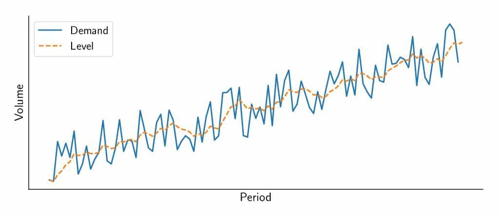
As you can observe, the exponential smoothing model will then forecast the future demands as its last estimation of the level.
The underlying idea of any exponential smoothing model is that, at each period, the model will learn a bit from the most recent demand observation and remember a bit from the last forecast made. The magic about this is that the last forecast the model made, includes a part of the previous demand observation and a part of the previous forecast. And so forth. Hence this previous forecast actually includes everything the model has learned so far based on demand history.
The smoothing parameter (or learning rate) alpha (\alpha) will determine how much importance is given to the most recent demand observation. Let's represent this mathematically:

    \[f_t=\alpha d_{t-1}+(1-\alpha) f_{t-1}\]


    \[0 < \alpha \leq 1\]

\alpha d_{t-1} represents the previous demand observation times the learning rate.
(1-\alpha) f_{t-1} represents how much the model remembers from its previous forecast.

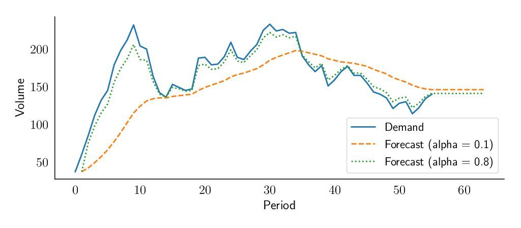
On the figure below, we see that a forecast made with a low alpha value (here 0.1) will take more time to react to a changing demand, whereas a forecast with a high alpha value (here 0.8) will closely follow the demand fluctuations. You can find more information about this model on supchains.com

An advantageous demand forecasting model and an important starting point

There are two key advantages to highlight on exponential smoothing:

• The weight associated with each observation decreases exponentially over time (the most recent observation has the highest weight).
• We can reduce the impact of outliers and noise thanks to alpha (α), the exponential weight.

As explained in the book “Data Science for Supply Chain Forecast” written by Nicolas Vandeput, there is an important trade-off to be made between learning and remembering; between being reactive and being stable. If the learning rate is high, the model will allocate more importance to the most recent demand observation and it will be reactive to a change in the demand level. But it will also be sensitive to outliers and noise. On the other hand if the learning rate is low, the model won't notice a change in level rapidly, but will also not overreact to noise and outliers.
But it also has some demand planning limitations to consider:

• The exponential smoothing model does not project trends, and it does not recognize any seasonal pattern.
• It cannot use any external information (such as pricing or marketing expenses).

Final thoughts on choosing a demand forecasting method

This first exponential smoothing model will be most likely too simple to achieve good results, but it is a good foundation on which to create more complex models later. To avoid some of the shortcomings described here, there are more advanced smoothing techniques that we describe in another blog post. Moreover, you can see these models applied to your data in SKU Science in order to compare them, and let our algorithm pick the best one for each forecast.

Try our fast & simple demand forecasting solution
Sign up for free to SKU Science today!
Pre-loaded sample data - No credit card required