Going through the concept to improve your demand planning process
Let’s first recapitulate. The Forecast (f) in double exponential smoothing is calculated by two layers, the Level (a) plus the Trend (b).

By inserting the seasonality into the model, Seasonal Factor (s), a new layer of exponential smoothing is added. It is estimated based on the most recent observation and its previous estimation.
A learning rate, gamma ( ), is applied to the Seasonal Factor (s) metric, so the model will use an exponential weighting method in order to determine how much weight percentage is given to the most recent observation compared to the previous estimation. In other words, gamma will determine if the forecast should respond quickly or not to a certain demand variation. Considering that seasonality in general doesn´t have significant changes from one year to another, keeping the learning rate low, lower than 0.3 for example, will avoid unnecessary adapting to fit exceptional situations and outliers, and will keep this method a more regularized forecast model.
Still, it may require some degree of understanding of your market demand, but knowing if your seasonality is monthly, quarterly or yearly based, should give you a good hint as to the best degree of learning rate to use.
Choosing the right method for accurate demand forecasting
The triple exponential smoothing technique has two different approaches, and you should know the nature of your seasonality, in order to know which one to use.
- Multiplicative Smoothing
If you sell 20% more of your product in December than in November, you probably have a multiplicative seasonal nature. In this case the Seasonal Factor (s) is simply multiplied into the forecast:

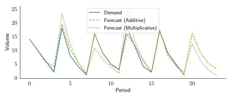
This predicts with reliable accuracy, responding in a very effective way to variations of seasonality and following the general trend of the demand, as shown on the example below comparing it with the forecast.
However, this method can result in mathematical errors if volumes or the seasonality factors are too close to 0. Also a small absolute demand variation can result in a great difference. Unfortunately, this means that this model is not suited for all products, and reinforces the importance of knowing the seasonal nature of your products.
In order to solve this issue a second demand forecasting approach is preferred:
- Additive Smoothing
If you sell 20,000 more of your products in December than in November you have an additive seasonal nature. With this approach a season factor is added to the level predicted by the forecast model, so that the forecast responds with more adherence even at low volumes. Now we add the Seasonal Factor (s) into the forecast: 
Putting both approaches into a visual graphic perspective, gives us a clearer idea of how they will react over the demand variation, showing a best fit for the additive model.