Manufacturing: 4 Keys to Smarter Demand Forecasting

Demand Forecasting in the Manufacturing Industry: Key Points to Master In the manufacturing industry, poor demand forecasting doesn’t just show up as a bad number in an Excel spreadsheet, it materializes as costly overstock, production stoppages, missed delivery deadlines, and unhappy customers. The stakes are concrete, immediate, and often massive. Yet many supply chain teams continue to manage their planning with inadequate tools or overly manual processes. So, how do you build a robust demand forecasting approach in a manufacturing context? Here are the key points to consider. 1. Understanding the Specifics of Manufacturing Demand Demand in the manufacturing industry doesn’t look like demand in distribution or retail. It has its own characteristics that make forecasting more complex: Long cycles and extended lead times: when a component’s lead time exceeds several weeks, mid-term forecast accuracy becomes critical. A mistake today is paid for dearly three months down the road. Largely derived demand: demand for raw materials or components depends directly on finished goods forecasts. This means forecasts must be cascaded through Bills of Materials (BOMs). Seasonality and promotional effects: sales campaigns, RFQs, or industrial cycles can create demand spikes that are hard to anticipate without the right data. A heterogeneous product portfolio: some items are predictable best-sellers, others are spare parts with sporadic or intermittent demand. No single forecasting method fits all. Recognizing these characteristics is the first step toward selecting the right forecasting models and best practices. 2. Choosing the Right Forecasting Methods Based on Demand Profiles One of the most common mistakes is applying a single method across the entire catalog. Yet every demand profile deserves a tailored approach. Regular, stable demand: exponential smoothing methods (Holt, Holt-Winters) deliver strong results in the vast majority of cases. They reliably capture trend and seasonality. Intermittent or sporadic demand: for spare parts or slow-moving SKUs, specialized methods such as Croston or Syntetos-Boylan can outperform classic moving averages. That said, given the difficulty of forecasting such demand, it’s better to focus your energy on inventory management. New products or launches: without historical data, you need to rely on analog references, market studies, or collaborative forecasts involving sales teams. Automation and machine learning: for portfolios spanning thousands of SKUs, automating forecasts through dynamically selected algorithms (based on past performance) is a major performance lever. The goal isn’t to use the most sophisticated method, it’s to use the most appropriate one for your business, with minimized and measurable forecast error. 3. Incorporating External Signals and Cross-Functional Collaboration Statistical algorithms, however powerful, cannot anticipate everything. In the manufacturing industry, ground-level intelligence carries significant value: Sales forecasts: sales teams hold valuable insight into active deals, pricing negotiations, or customer churn. These signals need to feed into the forecasting process. Customer data and firm orders: in a B2B context, order books or long-term contracts can dramatically reduce uncertainty over certain planning horizons. Macroeconomic and industry trends: industrial production indices, commodity prices, or sector-level activity can serve as useful leading indicators. The S&OP process (Sales & Operations Planning): structuring a monthly consensus meeting between sales, marketing, operations, and supply chain teams helps reconcile different perspectives and land on a single, shared forecast. Demand forecasting is not a siloed activity, it’s a cross-functional process that gains in accuracy when the whole organization contributes. 4. Measuring Performance and Driving Continuous Improvement An unmeasured forecast is an uncontrolled forecast. To improve, you need to put clear KPIs in place and track them consistently. MAE (Mean Absolute Error): MAE represents the average deviation between what you forecasted and what actually sold, regardless of the direction of the error (over- or under-forecast). Avoid MAPE, it encourages under-forecasting and blows up on low-volume items. Bias: measures whether forecasts are systematically over- or under-estimated. Persistent bias is the sign of a structural issue that needs to be corrected. Segment-level tracking: analyzing forecast accuracy by product family, sales channel, or planning horizon helps identify priority areas for improvement. Forecast Value Added (FVA): FVA is a performance metric that measures the effectiveness of each step in the forecasting process. Unlike MAE, which measures overall error, FVA answers a strategic question: “Did human intervention actually improve accuracy, or did we just waste time?” Beyond metrics, the goal is to build a culture of continuous improvement: analyzing significant variances, understanding their root causes (exceptional events, data entry errors, wrong model), and adjusting forecasts or processes accordingly. Conclusion: Turning Forecasting Into a Competitive Advantage In the manufacturing industry, demand forecasting is much more than a technical exercise, it’s a strategic lever. Better accuracy means less tied-up inventory, fewer stockouts, more stable production schedules, and ultimately, stronger profitability. The good news is that modern tools now make it possible to automate a large part of this work, test dozens of models in seconds, and focus team energy where it adds the most value: analysis, decision-making, and collaboration. Ready to take it further and improve your forecast accuracy starting now? Discover how SKU Science can help you industrialize your demand forecasting process — simply, quickly, and without a heavy IT project.
New Product Lifecycle Module: Seamless Product Transitions, Made Simple

Streamline your product transitions Automatically transfer historical data and preserve forecast accuracy Introduction Launching a new product or phasing one out should never feel like an uphill battle. Yet every phase-in or phase-out comes with risks: stockouts, excess inventory, lost revenue, and increased pressure on teams. All of this is often made worse by unreliable data at the very moment when decisions matter most. Our new Product Lifecycle Management module changes the game. It ensures smooth, controlled transitions with accurate forecasts available from day one. You can anticipate better, decide faster, and protect your performance with confidence. Navigating the challenges of product transitions Planners know it well: a poorly managed product transition can be costly. Here are the main pitfalls to avoid: Unmanaged end-of-life phases: excess inventory that ties up cash. Underestimated new product launches: missed sales opportunities from day one. Channel variability: different forecasts per country, store, or e-commerce channel that are difficult to replicate accurately. Lack of usable historical data: making it impossible to build reliable forecasts for new products. Manual updates: a major source of errors whenever a product code changes or marketing adjusts the timeline. The result is often the same: delayed decisions, reduced visibility, and reactive rather than strategic planning. An intelligent module to manage the entire product lifecycle Our new product lifecycle management module centralizes what planners previously had to handle manually. It connects end-of-life products with their successors while ensuring full continuity of forecasts. Each transition becomes transparent: you can clearly visualize the links between old and new products, manage transition timelines, and keep a complete history of changes. This approach provides full control over your product portfolio, from SKU creation to product retirement. Automating phase-in and phase-out processes One of the key strengths of the module lies in its automation capabilities.When a product reaches end of life, you simply assign its successor. The system automatically transfers the relevant data — including historical data and associated segments — to the new product. Forecasting models adapt seamlessly to real-life conditions: Automatic creation of forecasts for the successor product Dynamic transfer of historical data to ensure forecast continuity Preservation of links between products during the transition period (phase-in / phase-out) The result: fewer errors, smoother transitions, and stable forecasts — even when marketing calendars change. Advanced multi-channel forecasting management In many organizations, a single product can have multiple forecasts depending on sales channels, geographic regions, or customer segments. This level of granularity is essential, but often difficult to manage. Our module automates this complexity.For example, if a product has five separate forecasts by channel, the successor will automatically inherit all five. Each channel keeps its own sales dynamics, without manual duplication or data loss. This approach preserves local accuracy while significantly reducing operational workload. Creating new products based on existing ones Another common use case is launching a new product that has no direct predecessor but shares similar characteristics with an existing one.The module allows you to create a new product based on the data of an existing item, without establishing any formal link between them. This makes it easy to accelerate product launches while starting with reliable, experience-based forecasts. More reliable forecasts for better decision-making Thanks to these automations, product transitions become an opportunity rather than a constraint. You gain: Greater accuracy, with realistic forecasts from the very first planning cycles More agility, through instant creation of new products Peace of mind, as teams no longer need to manually manage hundreds of SKUs The results are tangible: reduced excess inventory, fewer stockouts, and improved visibility into future performance. Conclusion Product transitions should never put your sales plan at risk. With this new module, you can manage the entire product lifecycle from a single interface, without data loss or forecasting disruptions. Give your products the future they deserve. Discover the module in action and start managing your product lifecycle with confidence.
Reducing stockout impact with aggregate forecasting

Many companies do not have a process for archiving or tracking stockouts, even though they can have a significant impact on sales. This article will outline how organizations can minimize the effect of stockouts on demand forecasting through the use of aggregate forecast methods and actual sales data. While it would be preferable to use actual demand rather than historical sales by eliminating stockouts, our experience indicates that most companies have not yet reached this stage of maturity in their supply chain management. Free Trial – Fast & Simple demand forecasting solutionEasy and affordable – No credit card requiredTry SKU Science now ! SIGN UP FREE Benefits of using aggregated data for demand forecasting The best practice in supply chain management to achieve greater forecast accuracy is to calculate forecasts at an aggregate level. Here are some reasons why demand forecasting KPIs typically improve with this approach: – Increased sample size: By aggregating data from multiple sources, you increase the sample size of your data, which can improve the accuracy of your forecasts. A larger sample size can provide a more representative view of the population, allowing for more robust and reliable predictions. – Reduction of noise: Aggregating data can help reduce the effects of noise and outliers in the data. For example, if you’re forecasting demand for a product, an unusually high demand from a single customer or location might skew the data and lead to an inaccurate forecast. By aggregating data across multiple customers or locations, you can reduce the impact of these outliers and produce more accurate forecasts. – Better understanding of underlying patterns: Aggregating data can help you identify patterns and trends that you might not see when working with individual data points. For example, if you’re forecasting demand for a product across multiple stores, you might notice that demand tends to be higher on weekends or during certain months of the year. By identifying these patterns, you can create more accurate forecasts. – More explanatory power: Aggregating data can give you a more complete understanding of the factors that influence demand for a product or service. For example, by analyzing data from multiple stores, you may be able to identify both a seasonal pattern and store-specific characteristics that affect demand. Combining these two factors can provide more explanatory power and more accurate forecasts. Effective data grouping techniques for accurate demand forecasting Now let’s see what type of data we could use to group our data in order to apply our forecasting models. – Product data such as product size, weight, color, price, brand, segment, category, or any other field characterizing a product can be used to aggregate data. – Store data can also be used to understand how demand for a product varies across different store locations. This can include information such as store size, layout, and demographics of the surrounding area. – Sales channel is another example of information that can be used to organize your data before computing the forecast since the demand for specific channels can be very different. – Marketing data such as promotions or advertisements that were run for the product, can help understand the effect of these activities on demand. Therefore, grouping data using these fields or a combination of these fields can lead to better accuracy when forecasting demand. This table shows the average error rate in % for forecasts computed at a specific aggregate level Improving demand forecasting accuracy through aggregate data and stockout analysis If historical sales data is impacted by stockouts, it can lead to inaccuracies in demand forecasting because stockouts can cause fluctuations in sales that do not reflect true underlying demand. As seen earlier, working with aggregate data can help improve the accuracy of demand forecasting in this situation for a few reasons: – Smoothing effect: Aggregating sales data from multiple sources can help to smooth out fluctuations in sales caused by individual stockouts. For example, if sales data from one store is affected by a stockout, it can be offset by sales data from another store where stockouts did not occur. – Better understanding of the impact of stockouts: By aggregating data across multiple stores, you can also gain a better understanding of how stockouts are impacting demand. This can help you to identify which products are most affected by stockouts, as well as which stores or regions are more affected, you can use this information to plan and manage your inventory. – Reduced variability: Stockouts can cause significant variability in sales data, which can be especially problematic for statistical forecasting methods that rely on historical data. By aggregating data, you can help to reduce this variability, which can improve the accuracy of your forecasts. It’s important to note that even when working with aggregate data if stockouts are a frequent and persistent problem, it can make the forecasting process more challenging, and it’s important to consider ways to address the root causes of stockouts to improve forecast accuracy. Free Trial – Fast & Simple demand forecasting solutionEasy and affordable – No credit card requiredTry SKU Science now ! SIGN UP FREE Gains on forecasting KPIs for our customers As discussed earlier, there are several possible options for aggregating data to calculate the aggregate forecast, each with a specific error rate. It is important to consider several options and choose the most appropriate one for your needs. Forecast KPIs such as bias and error will help you identify the best level of aggregation for your calculations. However, it can be challenging to split aggregate forecast data into underlying forecasts for each period, which can be time-consuming and may result in inaccuracies. SKU Science has developed a fully automated feature that computes underlying forecasts for each period, making it easy to compare error rates and choose the relevant aggregate level. Our customers have been using this feature to lower their error rates and improve the accuracy of their demand forecasting. The impact can be significant, as we have seen up to 20%
Challenge your sales team’s forecasts with KPIs

To improve the performance of your supply chain, it is essential to have the right tools to support demand planning within your S&OP. Thus, you can limit stockouts and keep your inventory at a reasonable level while ensuring a high level of service. A key part of demand planning is getting the right forecast. Very often, these forecasts come from salespeople and distributors, however, the quality of these forecasts is frequently questioned by supply chain professionals. Focus on forecast KPIs for sales teams In practice, it is necessary to measure the quality of these forecasts (the famous KPIs). But it’s a difficult task to achieve with Excel. One can safely write, that there are as many ways of evaluating these forecasts that there are companies. We provide a performance tracking table below, to quickly identify items or levels in the organization requiring corrective action. SKU Science provides a solution to educate all players in the supply chain to improve forecasting. It is possible to recreate this table by hand in Excel, but it is a complicated task and requires monthly maintenance. Several customers have asked us to be able to compare the forecasts provided by their sales departments with those calculated by our platform.Hence, on this table, you can see 2 types of forecast. All the KPIs are calculated for the 2 two types of forecasts (depending on the lead times of your supply chain, otherwise it doesn’t make any sense) and compared to each other to calculate the added value of your sales team. Measure the forecast value-added of your teams Your teams spend time forecasting, but it only makes sense if they really improve the forecasting from a tool like SKU Science or some other platform. By comparing these data, you finally know if you are adding value, which must be your only goal. Concretely, how does this happen?From historical demand data, the platform computes forecasts for the last cycles. During each cycle, a new external forecast was uploaded from Excel onto the platform. These rolling forecasts from both the platform and sales representatives are archived at each new cycle. We analyze the forecast data with one month difference for each period in the example below.Instead of focusing on forecasts at the SKU level (you can own a lot of them), we study forecasts at a more macroscopic level, such as a territory or a warehouse (in this case Paris). This exercise is replicable at any level. The platform allows us to effortlessly obtain KPI tables calculated from quantities or financially valued. In the example below, a weighted KPI table is generated from the revenue of each SKU. This remains the best option to analyze KPIs and have a real impact on the company.Each calculated forecast KPI has 3 rows. • SKU Science: indicates the values concerning the platform forecasts.• User: indicates the values for the forecast from the sales department and uploaded to the platform.• Value added: represents the improvement or degradation made by the user compared to SKU Science. Forecast value-added and weighted KPIs It is easy to see in this table that the teams’ added value related to the forecast accuracy, in red, is 4% lower than the one obtained by the platform. Therefore, it is necessary to take corrective actions during the next cycles, to turn this figure into a positive. We will share some advice in another article to be successful. Without improvement in the next cycles, it is preferable not to change any platform’s forecasts and to avoid wasting your teams’ time. Another important piece of information that can be extracted from this table is the average difference between the actual turnover for each period and the forecast bias. Here we see, thanks to the negative sign, that the sales department underestimates on average $ 634k per month compared to the actual turnover. Shortages are to be feared on certain items in the Paris area without a good inventory policy. A positive sign would indicate a tendency to overestimate quantities, which would inevitably result in an increase in inventory level. The ideal situation would be to have a percentage bias close to zero. In general, it is good practice to analyze forecast KPIs against turnover or against the margin generated by the company.For some key articles, however, it may be interesting to analyze this table from the perspective of quantities. Free Trial – Fast & Simple demand forecasting solutionEasy and affordable – No credit card requiredTry SKU Science now ! SIGN UP FREE
How to set up a demand forecasting process

Forecasting demand is always a means to an end, not the end itself. A forecast is only relevant if it enables a supply chain to take appropriate actions. A good forecasting model should allow your supply chain to improve its service level, plan better, reduce waste, and overall costs. In this blog article, we introduce the 4-dimension demand forecasting framework to help you define the appropriate process for your organization. When setting up a demand forecasting process, you will have to set it across four dimensions: granularity, temporality, metrics, and process. 1. Granularity You should first work on determining the right geographical and material granularity for your forecast. ?️ Geographical. Should you forecast per country, region, market, channel, customer segment, warehouse, store? ? Material. Should you forecast per product, segment, brand, value, raw material required? To answer those questions, you have to think about the decisions taken by your supply chain based on this forecast. Remember, a forecast is only relevant if it helps your supply chain to take action. As an example, let’s assume you need to decide which products to ship from your plant to your regional warehouses. In that case, it might be a good idea to aggregate demand per each region allocated to a warehouse and forecast demand directly at this geographical level. To forecast the demand allocated to a warehouse, it is a bad practice to use historical orders as they are impacted by logistic constraints. Instead, you should forecast the warehouse demand based on what should be served from the warehouse if there were no constraints (in other words, forecast the demand coming from the geographical region that should be served by the warehouse). Free Trial – Fast & Simple demand forecasting solutionEasy and affordable – No credit card requiredTry SKU Science now ! SIGN UP FREE 2. Temporality Once you know at what granularity level you will be working on, you should pick the right forecasting horizon and temporal aggregation (time bucket). Many supply chains stick to forecast demand 18 or 24 months ahead, although you may need to pick a limited horizon to focus on. ?️ Temporal Aggregation. What temporal aggregation bucket should you use (day, week, month, quarter or year)? ? Horizon. How many periods do you need to forecast (one month, six months, two years)? Again, you should answer these questions by thinking about what your supply chain is trying to optimize/achieve and the lead times involved with these decisions. For example, let’s assume your suppliers (or production plants) need to receive monthly orders/forecasts three months in advance. In that case, you know you should work on monthly buckets and with a horizon of 3 months (M+1/+2/+3). You can also skip M+4 (or at least not focus on it). If you need a forecast to know what goods to ship from your central warehouse to your local warehouses, you should focus on a horizon equivalent to your internal lead time. ❗ Models and Forecasting Horizon. Statistical models can easily produce forecasts over a very long horizon (theoretically infinite). This is not the case with machine learning models. So, you might have to stick to statistical models for long-term forecasting. 3. Metrics Usually, practitioners overlook the question of forecasting metrics. Choosing the right metrics for a forecasting process/model is actually quite simple and will have profound impacts on the resulting forecasts. Depending on the metric selected, you might give too much importance to outliers (the RMSE flaw) or risk a biased forecast (the MAE flaw). Here are a few pieces of advice to choose the right forecasting metrics: ❌ Avoid MAPE. Many practitioners still use MAPE as a forecasting metric. This is a highly skewed indicator that will promote underforecasting. ✅ Combine KPIs. Choosing a combination of KPIs (such as MAE & Bias) will often be a good compromise enabling you to track accuracy and Bias while avoiding most pitfalls. ✅ Track consistent Bias. If a consistent bias (over/under forecasting) is observed on an item, something is probably wrong with the model/forecasting process. ? Weighted KPIs. You can try weighting each product (or SKU) in the overall metric calculation based on its profitability, cost, or overall supply chain impact. The idea is that you want to pay more attention to SKUs that matter the most. Beyond the math, it is important to align the forecasting KPIs to the required material and temporal granularities. For example, let’s assume you are interested in ordering goods from an overseas supplier with a lead time of 3 months. In that case, you should measure accuracy over a forecasting horizon at months +1,+2, and +3–or even better, calculate the cumulative error over three months–instead of merely looking at the accuracy achieved at month+1. 4. Demand forecasting process Now that you know your material and temporal aggregation, horizon, and metrics, you can set up a process. This process should be defined through three specific aspects. – Stakeholders. Who will review the forecast? Bringing different points of view to the table – using various information sources – will help create a more accurate forecast. – Periodicity. When do you review the forecast? Updating your forecast more often might improve its accuracy (as you have fresher data at hand). Updating it too often might create chaos as you overreact to demand changes and consume too many resources for a limited added value. – Review Process. How do you review the forecast? At the core of any forecasting process, there should be a measurement of the forecast value-added. Tracking each team member’s value-added will enable you to improve the forecasting process efficiency (and refine the relevant forecasting periodicity and stakeholders). ? Forecast Value Added Framework. A forecasting process framework that tracks each team/process step’s added value compared to a benchmark (or the previous team’s input). It was imagined and promoted by Michael Gilliland in the 2010s (see his book here). Our advice for your demand forecasting process – Short-term forecast. Let’s assume you need to decide every week what to
6 tips to get reliable demand forecasts post-COVID-19

The COVID-19 crisis has impacted all demand forecasting models, whatever your industry. Depending on the type of items you’re dealing with (low vs high demand) or your industry sector (retail, food, health care, utilities, logistic, manufacturing etc.), some measures need to be taken in order to plan (relatively) accurately for the months to come. The question is: “How should we treat actual demand data for March, April, and May 2020?” Demand during COVID-19 and its impact on the forecast model (Season & Trend model) Well, as you can imagine, there is not a single answer to this question, but we will try below to list all available options. We’re pretty sure that one will fit your business. The first obvious option is to tag these values as outliers. If you decide to treat March to May 2020 demand data as outliers, you then have several options for your forecast calculations. • You can remove them from the forecasting window. • You can implement some tactics to reduce their weight in your forecast models. • You can use historical data from previous years to replace these particular periods, by taking an average from 2017 – 2019 as an example. • You can use calculated forecast data from your model to replace these particular values. We will explain soon in another article how to quickly obtain your forecasts using this method with SKU Science. Demand during COVID-19 replaced with forecast data (Season & Trend model) Once your tactical choice is made – and taking into account that we are still in a VUCA world – you may consider allowing your forecast baseline to quickly adjust to changes in demand by increasing forecast parameters sensitivity. Dealing with Q1 and Q2, 2020 demand data will not just help you to properly plan for the rest of the year but also for Q1 and Q2, 2021. Indeed, for those with a seasonal demand, it is likely that your forecast models will “learn” a COVID-19 seasonality and predict a demand drop in March – May 2021. For some industries, flagging the lockdown months as outliers is not always the best option, because those sales could represent a new structural change that is likely to persist into the future – video conferencing solutions and medical teleconsultations spring to mind. Another example is an increased consumption of flour that could remain at this higher level in the months to come, as home cooking has gained the upper hand over fast food and eating out. Therefore, it is important for demand planners to know their industry so that they can properly interpret historical demand. In short, flagging recent demand as outliers is counterproductive if your customers have now changed their long-term behavior due to the crisis. Try our fast & simple demand forecasting solutionSign up for free to SKU Science today!Pre-loaded sample date – No credit card required SIGN UP FREE Another tactic to optimize your sales – while optimizing your working capital – would be to maintain low inventory levels for end products while maintaining a good level of raw material and WIP to allow for a rapid production ramp-up, in order to stay ahead if a demand increase arises. In conclusion, there is no forecasting silver bullet that is effective for all businesses. The demand over the last 3 months has been exceptional: it is likely that, in most cases, the post-COVID-19 demand will be different from the demand we have experienced during the last 3 months. Hence – except for some essential industries (e-commerce and food etc.) – it would be a safe bet to alter the demand data for March, April, and even May. If you currently use a statistical or a black-box algorithm it might be time to review how your forecast engine works to prevent it from overreacting to the COVID-19 crisis.
How to detect outliers for improved demand forecasting

Most supply chains expect some demand variability and therefore, one must choose the correct forecast model, as can be seen in our previous articles. Regardless of the nature of this variance, exceptional factors may happen, and can seriously impair the reliability of a given model. We call these data “outliers”. These outliers result firstly from exceptional demand, such as stock liquidations, temporary stops in production, or external restrictions, which may be due to logistical or infrastructural constraints making both the composition of the stock or the fulfillment of customer orders temporarily impossible. Even though some demand observations are real, it does not mean they are not exceptional and shouldn’t be cleaned Secondly, there are also mistakes and errors, which are obvious outliers. If you spot these kinds of errors or encoding mistakes, you need to implement process improvements in order to prevent them from happening again. Considering the negative effects outliers can bring to your business, knowing how to detect them is essential and there are some techniques that can be used to address this issue. Try our fast & simple demand forecasting solution Sign up for free to SKU Science today!Pre-loaded sample date – No credit card required SIGN UP FREE Winsorization This first idea is a rather simplistic approach of defining a certain minimum and maximum range in which the data will simply be disregarded. Statistically, this margin is defined as the percentile, which means the value below which x% of the observations in a group will fall. For example, 99% of the demand observations for a product will be lower than its 99th percentile. This approach may be efficient, but it can also result in some problems, such as detecting fake outliers in a dataset without outliers (see figure 1 below); or in the case of real outliers, it doesn’t sufficiently reduce the value keeping it at a level way above our expectation. It is an approach that ends up requiring a very accurate critical analysis by the planner, so it is not as efficient and reliable as it should be, as it would take out the high and low values of a dataset, even if they aren’t exceptional per se. Figure 1: Winsorization of a simple dataset without outlier Standard Deviation Another approach would be to use the demand variation around the historical average and exclude the values that are exceptionally far from this average, according to a certain range between two thresholds centered on the demand. Figure 2: Distance to the mean With this method, in a situation without outliers, we do not change any demand observation (we keep all values in this case), and in another situation with an outlier (see Y2 below), we do not change the low or high demand points but only the actual outlier (from 100 to 49 in the figure below). Figure 3: Outlier detection based on standard deviation (Normalization) Although it may seem to solve all the issues arising from the Winsorization approach, the actual limitation will arise when you have a product with a trend or seasonality. In this case, its historical average will not accurately represent the actual average for that given period, and consequently the thresholds may not correctly limit a possible outlier. Error standard deviation In order to solve the drawbacks from the Standard Deviation and Winsorization let’s go back to the definition of an outlier. An outlier is a value that you didn’t expect. In other words, it is a value far away from your prediction (i.e. your forecast). To spot outliers, we must therefore analyze the forecast error and see which periods are exceptionally wrong. If we compute the error for our forecast we would obtain a mean error and a standard deviation. You can refer to the book Data Science for Supply Chain Forecast, by Nicolas Vandeput to see real-life examples and more details. The figure below illustrates our results obtained from our forecast. Figure 4: Outlier detection via forecast error This smarter detection method, which analyzes the forecast error deviation instead of simply the demand variation around the mean, is able to flag the outliers much more precisely and reduce them back to a plausible value. Therefore, this should be your preferred method for accurate demand forecasting. Try our fast & simple demand forecasting solution Sign up for free to SKU Science today!Pre-loaded sample date – No credit card required SIGN UP FREE
Adding seasonality to demand forecasting

Seasonal products are common in many industries and can involve a large number of factors such as the influence of seasonal weather changes for example. By definition, it is any change at all that consistently influences your demand during the same periods. This places some complexity into demand forecasting models and limits the use of some of them. Simple and double exponential smoothing forecast models (discussed in previous articles) do not recognize these seasonal patterns and so cannot extrapolate any future seasonal behavior. Try our fast & simple demand forecasting solution Sign up for free to SKU Science today!Pre-loaded sample date – No credit card required SIGN UP FREE Going through the concept to improve your demand planning process Let’s first recapitulate. The Forecast (f) in double exponential smoothing is calculated by two layers, the Level (a) plus the Trend (b). By inserting the seasonality into the model, Seasonal Factor (s), a new layer of exponential smoothing is added. It is estimated based on the most recent observation and its previous estimation.A learning rate, gamma (), is applied to the Seasonal Factor (s) metric, so the model will use an exponential weighting method in order to determine how much weight percentage is given to the most recent observation compared to the previous estimation. In other words, gamma will determine if the forecast should respond quickly or not to a certain demand variation. Considering that seasonality in general doesn´t have significant changes from one year to another, keeping the learning rate low, lower than 0.3 for example, will avoid unnecessary adapting to fit exceptional situations and outliers, and will keep this method a more regularized forecast model. Still, it may require some degree of understanding of your market demand, but knowing if your seasonality is monthly, quarterly or yearly based, should give you a good hint as to the best degree of learning rate to use. Choosing the right method for accurate demand forecasting The triple exponential smoothing technique has two different approaches, and you should know the nature of your seasonality, in order to know which one to use. Multiplicative Smoothing If you sell 20% more of your product in December than in November, you probably have a multiplicative seasonal nature. In this case the Seasonal Factor (s) is simply multiplied into the forecast: This predicts with reliable accuracy, responding in a very effective way to variations of seasonality and following the general trend of the demand, as shown on the example below comparing it with the forecast. However, this method can result in mathematical errors if volumes or the seasonality factors are too close to 0. Also a small absolute demand variation can result in a great difference. Unfortunately, this means that this model is not suited for all products, and reinforces the importance of knowing the seasonal nature of your products.In order to solve this issue a second demand forecasting approach is preferred: Additive Smoothing If you sell 20,000 more of your products in December than in November you have an additive seasonal nature. With this approach a season factor is added to the level predicted by the forecast model, so that the forecast responds with more adherence even at low volumes. Now we add the Seasonal Factor (s) into the forecast: Putting both approaches into a visual graphic perspective, gives us a clearer idea of how they will react over the demand variation, showing a best fit for the additive model. But the additive method also has its demand forecasting limitations, such as an inability to deal with any external input (marketing budget or pricing impact for example). Besides that, there is the issue for items with a significant trend. The way the triple exponential smoothing model is defined, does not allow for the seasonality to quickly evolve through time nor to extrapolate changes. This new additive model is actually best suited for items with a stable demand or low demand. Going deeper into demand forecasting methods As you can see our two seasonal models are complementary and should allow you to forecast any seasonal product. However, achieving reliable results requires sensitive understanding of the behavior of your product demand variation over time. The best way of knowing which one you should use, is of course by experimenting.The concept of the triple model is not that complex, but delving deeply into the equations, may be a little complicated without the proper tools. For more information on this model and other exponential smoothing models, you can check the freely available, online reference book “Forecasting: Principles and Practice”, by Rob J Hyndman and George Athanasopoulos, two world-class leaders in the field of forecasting, and “Data Science for Supply Chain Forecast” by Nicolas Vandeput.SKU Science has all these models and tools and can provide all the support you need to apply these demand forecasting methods reliably and effectively to your demand planning process. You can also see a more detailed analysis of both models on supchains.com Try our fast & simple demand forecasting solution Sign up for free to SKU Science today!Pre-loaded sample date – No credit card required SIGN UP FREE
Improving demand planning with a double exponential smoothing model
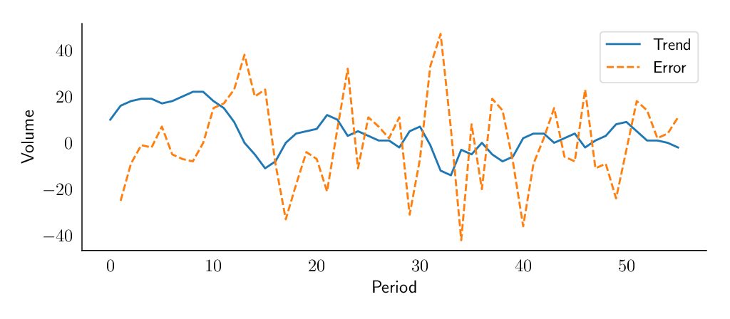
Accuracy in the demand forecasts for the Sales and Operations Planning (S&OP) process is extremely important and is fundamental to its success within a company. Some shortcomings found in simpler forecasting methodologies may undermine the credibility of your process. In this article we will explain how to solve some of the issues associated with the simple exponential smoothing model. As seen in a previous blog post, this model creates a simple forecast that assumes that future demand time series is similar to its past. A major issue with this simple smoothing is its inability to identify and project a trend. Try our fast & simple demand forecasting solution Sign up for free to SKU Science today!Pre-loaded sample date – No credit card required SIGN UP FREE We define the trend as the average variation of the time series level between two consecutive periods. In our November 2018 blog, the level is the average value around which the demand varies over time. So, for example, if you had a sales level last week of 10 pieces, and this week the sales level is around 20 pieces, this means that you have a positive trend of 10 pieces per week. If you assume that your time series follows a trend, most likely you will not know its magnitude in advance; especially as this magnitude could vary over time. However, there is now a model that can distinguish by itself the trend over time. As seen for the level, this new model will estimate the trend based on a new learning parameter called beta (), giving more or less importance to the most recent observations. Remember that alpha () will determine how much importance is given to the most recent demand observation. These demand forecasting techniques are now fully available to SKU Science, and we explain some of their key concepts below. Double exponential smoothing demand forecasting method at a glance The general idea behind double exponential smoothing models is that both level and trend will be updated at each period based on the most recent observation and the previous estimation of each component. As you may remember, with the simple exponential smoothing model, we updated the forecast at each period partially based on the previous demand and partially based on the previous forecast. We will now do the same for both level () and trend (). Our new demand forecasting model will update its estimation of the level at each period thanks to two pieces of information: the last demand observation and the previous level estimation increased by the trend. This demand forecasting model will also have to estimate the trend. Just as for the level, it represents how much weight is given to the most recent level observation. As soon as we are out of the historical demand period, we simply forecast each period as the last forecast plus the trend, and so the model will extrapolate the latest trend it has observed. However, as we will see later, this might present a problem. You can see below the mathematical representation for the forecasting technique: Level Estimation: Trend Estimation: Future Forecast: Initialization of our demand forecasting model As seen with the forecast initialization of the simple exponential smoothing, we have to discuss how to initialize the first estimations of our level and trend, and we will have two options as depicted below. Simple initialization We can initialize the level and the trend simply based on and .. This is a simple and fair initialization method. Linear regression Another way to initialize and would be to do a linear regression of the first n demand observations, that could be defined as an arbitrarily rather low number (e.g. 3 or 5). How to do linear regressions is out of scope for this article. Insights on these demand forecasting models Exponential smoothing models are very useful as they allow us to understand a forecast or a time series thanks to their decomposition between the level and the trend and (as we will see in another blog post), the seasonality. One can check the state of any of the demand sub-components at any point in time, just as you might check what is happening under the hood of a car. On the example below, we’ve plotted these different components to show you how our model understands a specific product. It explains why our model forecasts a specific value. The value of the different smoothing parameters will also tell you something about the variability or smoothness of your product. High values will denote a product where each variation should have an impact on the forecast; low values will denote products with a more constant behavior that should not be impacted by short-term fluctuations. The value of the different smoothing parameters will also tell you something about the variability or smoothness of your product. High values will denote a product where each variation should have an impact on the forecast; low values will denote products with a more constant behavior that should not be impacted by short-term fluctuations. Limitations of the double exponential smoothing demand forecasting model Our double exponential smoothing model is now able to recognize a trend and extrapolate it into the future. This is a major improvement compared to simple exponential smoothing or moving average. But, unfortunately, this comes with a risk. Our model will assume that the trend will go on forever. This might result in some issues for mid/long-term forecasts. We will solve this thanks to the damped trend model – a model that was published 25 years ago, in 1985! Next to the risk of infinite trend, we still have The lack of seasonality. This will be solved via the triple exponential smoothing model detailed in our next blog post. The impossibility of taking external information into account (such as marketing budget or price variations). Improving the forecasting technique with a damped trend To solve part of these limitations, Gardner and McKenzie (1985) proposed adding a new layer of intelligence: a damping factor phi () that
How to pick the best demand forecasting method to improve demand planning
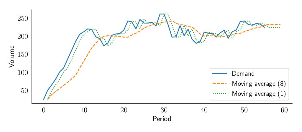
Future demand forecast is the basis for all strategic and planning decisions in a supply chain. A company defines its efforts according to the direction its business will go, which may be determined by basing it on a proper demand forecasting method. Additionally, it is the basis for a sales and operations planning (S&OP) process that covers production, sales, marketing, and finance areas, to allow managers to properly direct and align their actions that are data-driven rather than based on individual assumptions. Try our fast & simple demand forecasting solution Sign up for free to SKU Science today!Pre-loaded sample date – No credit card required SIGN UP FREE To successfully follow this approach and to ensure reliable results, managers must make important decisions on what to predict, and on the correct type of demand forecasting technique. Different techniques are available, but with substantial differences between them that should be chosen taking into account several factors. Since most techniques are quantitative, these factors must include the level of complexity of products or market, the maturity of the company supply chain processes, and the availability of reliable data.Two well-known basic demand forecasting techniques, that could be taken as a starting point use historical data to predict the future, but with some differences that will be descrambled below. The moving average demand forecasting model The first and the most basic is the moving average model, a demand forecasting method based on the idea that future demand is similar to the recent demand observed. In this model it is simply assumed that the forecast is the average of the demand during the last n periods. If you look at the demand on a monthly basis, this could translate as “We predict the demand in June to be the average of March, April and May”. In this way, a basic condition of the model is to start creating a historical database, as you won’t have a forecast until enough demand observations have been collected. Once out of the historical period, you simply define any future forecast as the last one made based on historical demand. That means with this model, the future demand forecast will be flat, thus one of the major restrictions of this model will be its inability to extrapolate any trend. Exponential smoothing demand forecasting model As for the moving average, it is assumed that the future will be more or less the same as the past. Similarly, the exponential smoothing model will be able to learn the level from demand history. The level is the average value around which the demand varies over time. It is important to understand that there is no definitive mathematical definition of the level; instead it is up to our model to estimate it. As you can observe, the exponential smoothing model will then forecast the future demands as its last estimation of the level. The underlying idea of any exponential smoothing model is that, at each period, the model will learn a bit from the most recent demand observation and remember a bit from the last forecast made. The magic about this is that the last forecast the model made, includes a part of the previous demand observation and a part of the previous forecast. And so forth. Hence this previous forecast actually includes everything the model has learned so far based on demand history. The smoothing parameter (or learning rate) alpha ($alpha$) will determine how much importance is given to the most recent demand observation. Let’s represent this mathematically: represents the previous demand observation times the learning rate. represents how much the model remembers from its previous forecast. On the figure below, we see that a forecast made with a low alpha value (here 0.1) will take more time to react to a changing demand, whereas a forecast with a high alpha value (here 0.8) will closely follow the demand fluctuations. You can find more information about this model on supchains.com An advantageous demand forecasting model and an important starting point There are two key advantages to highlight on exponential smoothing: • The weight associated with each observation decreases exponentially over time (the most recent observation has the highest weight). • We can reduce the impact of outliers and noise thanks to alpha (α), the exponential weight. As explained in the book “Data Science for Supply Chain Forecast” written by Nicolas Vandeput, there is an important trade-off to be made between learning and remembering; between being reactive and being stable. If the learning rate is high, the model will allocate more importance to the most recent demand observation and it will be reactive to a change in the demand level. But it will also be sensitive to outliers and noise. On the other hand if the learning rate is low, the model won’t notice a change in level rapidly, but will also not overreact to noise and outliers. But it also has some demand planning limitations to consider: • The exponential smoothing model does not project trends, and it does not recognize any seasonal pattern. • It cannot use any external information (such as pricing or marketing expenses). Final thoughts on choosing a demand forecasting method This first exponential smoothing model will be most likely too simple to achieve good results, but it is a good foundation on which to create more complex models later. To avoid some of the shortcomings described here, there are more advanced smoothing techniques that we describe in another blog post. Moreover, you can see these models applied to your data in SKU Science in order to compare them, and let our algorithm pick the best one for each forecast. Try our fast & simple demand forecasting solution Sign up for free to SKU Science today!Pre-loaded sample date – No credit card required SIGN UP FREE