Adding seasonality to demand forecasting

Seasonal products are common in many industries and can involve a large number of factors such as the influence of seasonal weather changes for example. By definition, it is any change at all that consistently influences your demand during the same periods. This places some complexity into demand forecasting models and limits the use of some of them. Simple and double exponential smoothing forecast models (discussed in previous articles) do not recognize these seasonal patterns and so cannot extrapolate any future seasonal behavior. Try our fast & simple demand forecasting solution Sign up for free to SKU Science today!Pre-loaded sample date – No credit card required SIGN UP FREE Going through the concept to improve your demand planning process Let’s first recapitulate. The Forecast (f) in double exponential smoothing is calculated by two layers, the Level (a) plus the Trend (b). By inserting the seasonality into the model, Seasonal Factor (s), a new layer of exponential smoothing is added. It is estimated based on the most recent observation and its previous estimation.A learning rate, gamma (), is applied to the Seasonal Factor (s) metric, so the model will use an exponential weighting method in order to determine how much weight percentage is given to the most recent observation compared to the previous estimation. In other words, gamma will determine if the forecast should respond quickly or not to a certain demand variation. Considering that seasonality in general doesn´t have significant changes from one year to another, keeping the learning rate low, lower than 0.3 for example, will avoid unnecessary adapting to fit exceptional situations and outliers, and will keep this method a more regularized forecast model. Still, it may require some degree of understanding of your market demand, but knowing if your seasonality is monthly, quarterly or yearly based, should give you a good hint as to the best degree of learning rate to use. Choosing the right method for accurate demand forecasting The triple exponential smoothing technique has two different approaches, and you should know the nature of your seasonality, in order to know which one to use. Multiplicative Smoothing If you sell 20% more of your product in December than in November, you probably have a multiplicative seasonal nature. In this case the Seasonal Factor (s) is simply multiplied into the forecast: This predicts with reliable accuracy, responding in a very effective way to variations of seasonality and following the general trend of the demand, as shown on the example below comparing it with the forecast. However, this method can result in mathematical errors if volumes or the seasonality factors are too close to 0. Also a small absolute demand variation can result in a great difference. Unfortunately, this means that this model is not suited for all products, and reinforces the importance of knowing the seasonal nature of your products.In order to solve this issue a second demand forecasting approach is preferred: Additive Smoothing If you sell 20,000 more of your products in December than in November you have an additive seasonal nature. With this approach a season factor is added to the level predicted by the forecast model, so that the forecast responds with more adherence even at low volumes. Now we add the Seasonal Factor (s) into the forecast: Putting both approaches into a visual graphic perspective, gives us a clearer idea of how they will react over the demand variation, showing a best fit for the additive model. But the additive method also has its demand forecasting limitations, such as an inability to deal with any external input (marketing budget or pricing impact for example). Besides that, there is the issue for items with a significant trend. The way the triple exponential smoothing model is defined, does not allow for the seasonality to quickly evolve through time nor to extrapolate changes. This new additive model is actually best suited for items with a stable demand or low demand. Going deeper into demand forecasting methods As you can see our two seasonal models are complementary and should allow you to forecast any seasonal product. However, achieving reliable results requires sensitive understanding of the behavior of your product demand variation over time. The best way of knowing which one you should use, is of course by experimenting.The concept of the triple model is not that complex, but delving deeply into the equations, may be a little complicated without the proper tools. For more information on this model and other exponential smoothing models, you can check the freely available, online reference book “Forecasting: Principles and Practice”, by Rob J Hyndman and George Athanasopoulos, two world-class leaders in the field of forecasting, and “Data Science for Supply Chain Forecast” by Nicolas Vandeput.SKU Science has all these models and tools and can provide all the support you need to apply these demand forecasting methods reliably and effectively to your demand planning process. You can also see a more detailed analysis of both models on supchains.com Try our fast & simple demand forecasting solution Sign up for free to SKU Science today!Pre-loaded sample date – No credit card required SIGN UP FREE
Improving demand planning with a double exponential smoothing model
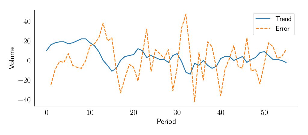
Accuracy in the demand forecasts for the Sales and Operations Planning (S&OP) process is extremely important and is fundamental to its success within a company. Some shortcomings found in simpler forecasting methodologies may undermine the credibility of your process. In this article we will explain how to solve some of the issues associated with the simple exponential smoothing model. As seen in a previous blog post, this model creates a simple forecast that assumes that future demand time series is similar to its past. A major issue with this simple smoothing is its inability to identify and project a trend. Try our fast & simple demand forecasting solution Sign up for free to SKU Science today!Pre-loaded sample date – No credit card required SIGN UP FREE We define the trend as the average variation of the time series level between two consecutive periods. In our November 2018 blog, the level is the average value around which the demand varies over time. So, for example, if you had a sales level last week of 10 pieces, and this week the sales level is around 20 pieces, this means that you have a positive trend of 10 pieces per week. If you assume that your time series follows a trend, most likely you will not know its magnitude in advance; especially as this magnitude could vary over time. However, there is now a model that can distinguish by itself the trend over time. As seen for the level, this new model will estimate the trend based on a new learning parameter called beta (), giving more or less importance to the most recent observations. Remember that alpha () will determine how much importance is given to the most recent demand observation. These demand forecasting techniques are now fully available to SKU Science, and we explain some of their key concepts below. Double exponential smoothing demand forecasting method at a glance The general idea behind double exponential smoothing models is that both level and trend will be updated at each period based on the most recent observation and the previous estimation of each component. As you may remember, with the simple exponential smoothing model, we updated the forecast at each period partially based on the previous demand and partially based on the previous forecast. We will now do the same for both level () and trend (). Our new demand forecasting model will update its estimation of the level at each period thanks to two pieces of information: the last demand observation and the previous level estimation increased by the trend. This demand forecasting model will also have to estimate the trend. Just as for the level, it represents how much weight is given to the most recent level observation. As soon as we are out of the historical demand period, we simply forecast each period as the last forecast plus the trend, and so the model will extrapolate the latest trend it has observed. However, as we will see later, this might present a problem. You can see below the mathematical representation for the forecasting technique: Level Estimation: Trend Estimation: Future Forecast: Initialization of our demand forecasting model As seen with the forecast initialization of the simple exponential smoothing, we have to discuss how to initialize the first estimations of our level and trend, and we will have two options as depicted below. Simple initialization We can initialize the level and the trend simply based on and .. This is a simple and fair initialization method. Linear regression Another way to initialize and would be to do a linear regression of the first n demand observations, that could be defined as an arbitrarily rather low number (e.g. 3 or 5). How to do linear regressions is out of scope for this article. Insights on these demand forecasting models Exponential smoothing models are very useful as they allow us to understand a forecast or a time series thanks to their decomposition between the level and the trend and (as we will see in another blog post), the seasonality. One can check the state of any of the demand sub-components at any point in time, just as you might check what is happening under the hood of a car. On the example below, we’ve plotted these different components to show you how our model understands a specific product. It explains why our model forecasts a specific value. The value of the different smoothing parameters will also tell you something about the variability or smoothness of your product. High values will denote a product where each variation should have an impact on the forecast; low values will denote products with a more constant behavior that should not be impacted by short-term fluctuations. The value of the different smoothing parameters will also tell you something about the variability or smoothness of your product. High values will denote a product where each variation should have an impact on the forecast; low values will denote products with a more constant behavior that should not be impacted by short-term fluctuations. Limitations of the double exponential smoothing demand forecasting model Our double exponential smoothing model is now able to recognize a trend and extrapolate it into the future. This is a major improvement compared to simple exponential smoothing or moving average. But, unfortunately, this comes with a risk. Our model will assume that the trend will go on forever. This might result in some issues for mid/long-term forecasts. We will solve this thanks to the damped trend model – a model that was published 25 years ago, in 1985! Next to the risk of infinite trend, we still have The lack of seasonality. This will be solved via the triple exponential smoothing model detailed in our next blog post. The impossibility of taking external information into account (such as marketing budget or price variations). Improving the forecasting technique with a damped trend To solve part of these limitations, Gardner and McKenzie (1985) proposed adding a new layer of intelligence: a damping factor phi () that
How to pick the best demand forecasting method to improve demand planning
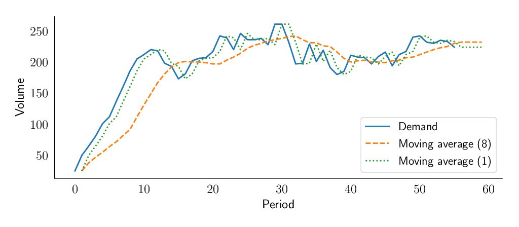
Future demand forecast is the basis for all strategic and planning decisions in a supply chain. A company defines its efforts according to the direction its business will go, which may be determined by basing it on a proper demand forecasting method. Additionally, it is the basis for a sales and operations planning (S&OP) process that covers production, sales, marketing, and finance areas, to allow managers to properly direct and align their actions that are data-driven rather than based on individual assumptions. Try our fast & simple demand forecasting solution Sign up for free to SKU Science today!Pre-loaded sample date – No credit card required SIGN UP FREE To successfully follow this approach and to ensure reliable results, managers must make important decisions on what to predict, and on the correct type of demand forecasting technique. Different techniques are available, but with substantial differences between them that should be chosen taking into account several factors. Since most techniques are quantitative, these factors must include the level of complexity of products or market, the maturity of the company supply chain processes, and the availability of reliable data.Two well-known basic demand forecasting techniques, that could be taken as a starting point use historical data to predict the future, but with some differences that will be descrambled below. The moving average demand forecasting model The first and the most basic is the moving average model, a demand forecasting method based on the idea that future demand is similar to the recent demand observed. In this model it is simply assumed that the forecast is the average of the demand during the last n periods. If you look at the demand on a monthly basis, this could translate as “We predict the demand in June to be the average of March, April and May”. In this way, a basic condition of the model is to start creating a historical database, as you won’t have a forecast until enough demand observations have been collected. Once out of the historical period, you simply define any future forecast as the last one made based on historical demand. That means with this model, the future demand forecast will be flat, thus one of the major restrictions of this model will be its inability to extrapolate any trend. Exponential smoothing demand forecasting model As for the moving average, it is assumed that the future will be more or less the same as the past. Similarly, the exponential smoothing model will be able to learn the level from demand history. The level is the average value around which the demand varies over time. It is important to understand that there is no definitive mathematical definition of the level; instead it is up to our model to estimate it. As you can observe, the exponential smoothing model will then forecast the future demands as its last estimation of the level. The underlying idea of any exponential smoothing model is that, at each period, the model will learn a bit from the most recent demand observation and remember a bit from the last forecast made. The magic about this is that the last forecast the model made, includes a part of the previous demand observation and a part of the previous forecast. And so forth. Hence this previous forecast actually includes everything the model has learned so far based on demand history. The smoothing parameter (or learning rate) alpha ($alpha$) will determine how much importance is given to the most recent demand observation. Let’s represent this mathematically: represents the previous demand observation times the learning rate. represents how much the model remembers from its previous forecast. On the figure below, we see that a forecast made with a low alpha value (here 0.1) will take more time to react to a changing demand, whereas a forecast with a high alpha value (here 0.8) will closely follow the demand fluctuations. You can find more information about this model on supchains.com An advantageous demand forecasting model and an important starting point There are two key advantages to highlight on exponential smoothing: • The weight associated with each observation decreases exponentially over time (the most recent observation has the highest weight). • We can reduce the impact of outliers and noise thanks to alpha (α), the exponential weight. As explained in the book “Data Science for Supply Chain Forecast” written by Nicolas Vandeput, there is an important trade-off to be made between learning and remembering; between being reactive and being stable. If the learning rate is high, the model will allocate more importance to the most recent demand observation and it will be reactive to a change in the demand level. But it will also be sensitive to outliers and noise. On the other hand if the learning rate is low, the model won’t notice a change in level rapidly, but will also not overreact to noise and outliers. But it also has some demand planning limitations to consider: • The exponential smoothing model does not project trends, and it does not recognize any seasonal pattern. • It cannot use any external information (such as pricing or marketing expenses). Final thoughts on choosing a demand forecasting method This first exponential smoothing model will be most likely too simple to achieve good results, but it is a good foundation on which to create more complex models later. To avoid some of the shortcomings described here, there are more advanced smoothing techniques that we describe in another blog post. Moreover, you can see these models applied to your data in SKU Science in order to compare them, and let our algorithm pick the best one for each forecast. Try our fast & simple demand forecasting solution Sign up for free to SKU Science today!Pre-loaded sample date – No credit card required SIGN UP FREE
How to get your S&OP Process right

Within the flow of a company’s supply chain planning process, the breakdown of functional silos and the integration of the various business areas involved, have long been endorsed. However, even with the adoption of integrated management systems, achieving tangible and quantifiable results remains a challenge for most companies. Within this scenario, companies are increasingly implementing the Sales and Operations Planning (S&OP) process, using straightforward practices that aim to simultaneously achieve improvements in terms of cost (inventory levels and cost of production) and service (product availability). These overall results are achieved by improving the sales and production planning process, based on a balance not only between demand and product availability (encompassing production and supplies) , but also between volume and product mix. Critical Success Factors S&OP is basically a fairly simple process, that encompasses two activities – demand forecasting methods and inventory planning – already discussed at meetings and carried out by a company. However, to be successful, the S&OP process requires a combination of factors to be implemented, as follows: Commitment of the company The first aspect to be considered concerns the degree of effective involvement of the company’s management body in the S&OP process. How often are managers present at meetings and what is their level of interaction when it comes to decision-makings?The second aspect concerns the involvement of all areas directly or indirectly affected by the material inventory planning process. As an example of an indirectly related area, we can cite maintenance or engineering. In some cases, changes from scheduled downtime to maintenance may be necessary to free up production capacity in order to meet the demand planning. Based on this example, it is possible to identify the importance of not only the presence of all areas with some relation to material requirements planning, but also that managers in these areas have the authority to make decisions. Meeting Planning Due to the many unfolding events that can impact sales and production planning, S&OP meetings are very often subject to lack of focus and to discussions about specific and less relevant points. Thus, meetings should be planned in such a way as to follow a set agenda for the main points to be discussed in order to prevent minor issues gaining undue importance. Try our fast & simple demand planning solution Sign up for free to SKU Science today!Pre-loaded sample date – No credit card required SIGN UP FREE Definition of responsibilities In addition to clarifying the responsibilities of the managers of each area within the process, it is advisable to designate a sponsor and a person responsible for the S&OP process as a whole. It is the sponsor’s responsibility to keep the entire company’s attention on the process; to remove possible impediments to incorporate necessary additional resources (participation of new people, or acquisition of supporting tools), and finally, to provide general support to the process. With respect to the person in charge of the process, their main responsibility is to manage the execution of each stages of the process, including the fulfillment of the defined deadlines, and to conduct planning meetings. Planning horizon This relates not only to the total planning period, but also to the point at which planning becomes more detailed (for example, planning for five months, but detailing the production mix for the next month only), and the presence or absence of a frozen planning period. The importance of these definitions is based on the specific need for planning by each area involved. For example, the supply area may require demand planning for three months due to purchase constraints, while production may be indifferent to the long-term, but requires a plan for the next month due to its production scheduling. Supporting tools In any planning process that requires some demand forecasting techniques, the use of digital resources and data models is a strong indication that the decisions made adequately take into consideration all trade-offs involved in the problem. For example, there is room to optimize some forecast models by applying several demand planning tools, and using software that enables more accuracy, transparency and agility during the process.It is worth noting that the use of support tools for each of the planning activities does not depend on the existence of an S&OP process, which may occur before or after the implementation of the S&OP process. The use of these tools, together with the S&OP process, has the effect of amplifying their potentialities; migrating from obtaining local gains to an integrated gain in planning efficiency. Financial follow-up S&OP meetings can be used to monitor and review the company’s overall budget, not only from a volume standpoint but also from revenue and profitability. This influence on the financial aspect occurs through possible changes in the planning of the sales mix. In this way, it is advisable to evaluate the impact of all planning alternatives discussed throughout the meetings. This evaluation can be carried out before the actual meeting, or even during the meeting, which gives greater flexibility and dynamics to the process. However, it does require a higher level of efficiency from decision support tools. Documentation of the process The degree of formalization of an S&OP process usually has a strong relationship with the documentation level of the process. Thus successful processes are expected to have a documented detailed planning policy that includes the participants, the responsibilities, the deadlines, and the objectives for each step of the process. Performance Monitoring In line with the financial monitoring aspect, monitoring the S&OP process should address both the performance as a whole, as well as the activities of each area involved in the process that may have an impact on its final performance.From the point of view of the final outcome of the process, it is important to monitor the availability of products for sales and inventory levels, in addition, of course, to the financial results of the company as a whole discussed above. In this respect, it is advisable to use a proper supply chain dashboard. With regard to